Processing Thermal Imagery

Introduction:

The definition of light that comes to the minds of most people is typically only limited to the visible spectrum. However, using thermal sensors, it is possible to record heat emitted as light. Thermal imagery has numerous applications, including locating of poorly insulated areas on rooftops, and mineral identification. By using a thermal sensor, your data capturing capabilities truly enter a whole new world (Figure 1).

Figure 1: An average reaction upon realizing the capabilities of thermal UAS imagery.

Methods:

The thermal camera captures images using the Portable Network Graphics (PNG) lossless compression. PNG is a fantastic method for recording raster data, however, Pix4D doesn't allow for PNG files to be entered as inputs, so it was necessary to convert the images from PNG into the TIFF file format. After the images were converted they were processed using Pix4D, generating a DSM and an orthomosaic.

Results:

The thermal imagery facilitated the creation of temperature maps, which allowed for the identification of specific features (Figure 2). The imagery was captured in the afternoon, which allowed the ground and vegetation to warm up. Water has higher thermal inertia than ground and vegetation, so water-covered areas appear dark blue.

Figure 2: The output Mosaic of the thermal imagery.

Figure 3: The pond and stream are visible in dark blue in the center of the image.

As water flowed from the pond, it traveled through a concrete culvert below to a lower pond. The culvert caused the surface temperature to drop, and it is easily visible in the bottom center of figure 3. Note how the concrete on the southern end appears warmer because it had been in direct sun (Figures 3, 4).

Figure 4: The culvert from the NE. 

Conclusion:

There are numerous untapped possible uses for thermal imaging, and this has been only one of them. In the future, I will pursue these additional uses.

Obliques and Merge for 3D model Construction

Introduction:

All of the imagery processed for this class up to this point has been captured from Nadir (pointing straight at the ground). Imagery captured at nadir is fantastic for the creation of orthomosaics and DSMs, but does not create aesthetically appealing 3D models. For 3D model creation, imagery captured at nadir and at oblique angles need to be fused into the same project.

Methods:

First, I ran the initial processing on the farm nadir flight, as well as the initial processing for the barn oblique flight. Next, I merged the two projects in Pix4D and ran the initial processing. After the initial processing, I noticed the flights had a 3m vertical offset between them, so I created two manual tie points, which re-aligned them into the same vertical plane.

Results:

The merged point cloud showed considerably more detail than the nadir generated orthomosaic.

Figure 1: 

Conclusion:

Oblique imagery provides increased detail to 3D models, however, the increased detail isn't necessarily worth the increased processing time.

Adding GCPs to Pix4D software

Introduction:

When Pix4D performs bundle-block adjustment on aerial images, the horizontal and vertical accuracy are dependent on the on-board GPS. Dependence on the on-board GPS can cause distortion of the resulting products. By recording the positions of features within the study area, it is possible to rectify the bundle-block adjustment to the known points and thus reduce distortion.

Methods:

In order to add GCPs to my project, I created a new project, imported my images, added their geolocation information, and had Pix4D use the default 3D maps preset. Next, I imported the GCPs using the "GCP/ Manual Tie Point Manager". After they were imported, I ran the project's initial processing. Once the initial processing was completed, I used the "GCP/ Manual Tie Point Manager" to identify the GCPs locations on the individual images. After the GCPs were identified, I ran the point cloud densification and orthomosaic generation steps.

After the orthomosaic and DSM were generated for the first project, I created a second project using the same images and same parameters, without using GCPs. Once the second project's orthomosaic and DSM were generated, I brought the products of both projects into ArcGIS in order to see how their accuracy differed.

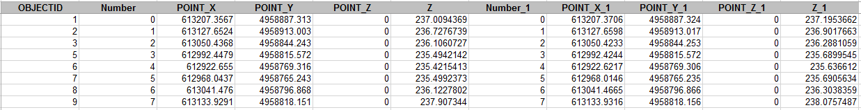
The first step was to digitize the GCPs locations on each output orthomosaic in two separate feature classes. Next, I used the "Add XY coordinates" tool to append each point's coordinates to its attribute table. I used the "Add Surface Information" tool to add the Z value for each point's location on its respective DSM to the attribute table. Once each the coordinates were added to each feature, I used the "Join" tool to combine the tables, then used the "Table to Excel" tool to export the combined table (Table 1). Next, I opened the table in Excel, where I calculated RMSE and the average 3-D distance between the two points (Tables 2,3).

Results:

Table 1: The output from the Table to Excel tool.

Table 2: The distance between the GCP locations on the images generated
with and without the use of GCPs

Table 3: The total 3-Dimensional distance between the locations in table 1.

Table 4: The horizontal RMSE, vertical RMSE, and average value for table 3.

The error between the two surfaces was rather minor, yet noticeable in certain parts of the images. The horizontal RMSE was 1.406 cm, slightly less than its pixel size of 1.666cm (Table 4). The vertical RMSE was substantially higher, at 18.78cm.

Image 1: The locations of the GCPs throughout Litchfield Mine.

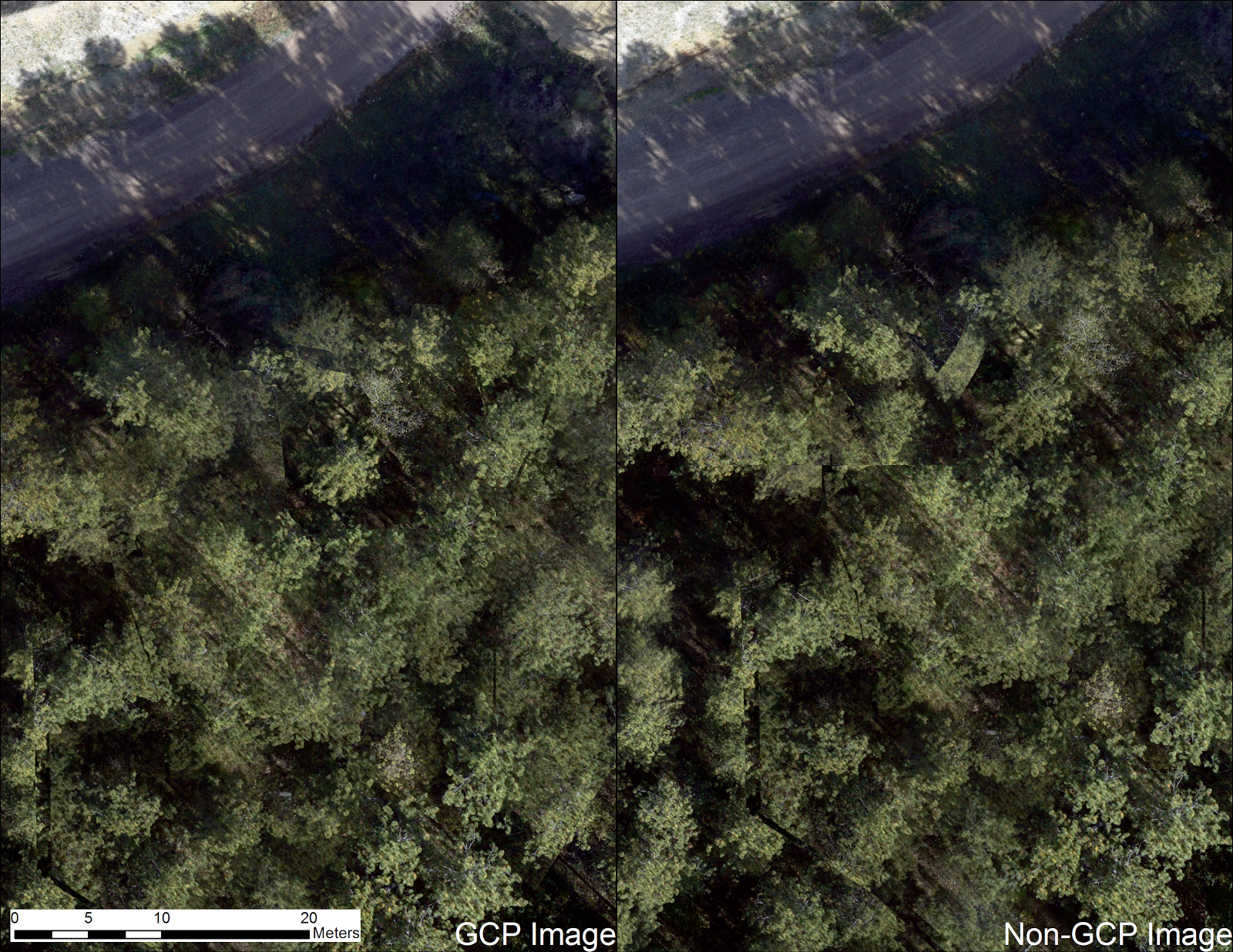
The images appeared identical at first, but closer inspection revealed discrepancies between the two (Image 2).

Image 2: Notice the discrepancy between the two images 1/3rd from the top of the image. 

Vertical error in the DSM increased as the distance from GCPs increased (Image 3).

Image 3: Elevation error and GCP locations.

At first I believed this increase in error was caused by the distance, but upon further inspection it seems the error is related to the type of feature (Image 4).

Image 4: Elevation error and feature type.

Conclusion:

The RMSE calculations indicated Pix4D's mosaics generated without GCPs have horizontal error less than the pixel size. This will be very useful for helping determine when GCPs are necessary in the future. The high vertical RMSE from the Non-GCP imagery, indicates that GCPs are truly important when recording elevation.