Introduction:
When Pix4D performs bundle-block adjustment on aerial images, the horizontal and vertical accuracy are dependent on the on-board GPS. Dependence on the on-board GPS can cause distortion of the resulting products. By recording the positions of recognizable features within the study area, it is possible to rectify the bundle-block adjustment to the known points and thus reduce distortion. For these points to be effective, the image analyst needs to be able to identify the exact location of the control point.
Methods:
The Litchfield mine site has been used for several of the previous labs, so it seemed prudent to place permanent GCP markers around the location, to ensure the accuracy of future flights. The markers were constructed of black plastic, commonly used to make the 'boards' surrounding hockey rinks. The plastic is flexible and weatherproof, so they should survive the elements, as well as any vehicles running them over. The GCP markers were spray painted with bright yellow spray paint, so a large 'X' is visible in the center of the marker. This 'X' will allow the analyst to precisely identify the point later when performing bundle block adjustment. After marking the 'X' on all of the markers, they were each labeled with individual letters of the alphabet, so they may be more easily identified in the field during later data collection.
On April 11, 2016, we travelled to the Litchfield site, and placed the GCP markers around the site. Before placing the markers, we removed sticks and flattened the soil/rock-material to ensure they aren't moved by wind. All of the selected locations had good aerial visibility, and were outside of well-travelled areas. The markers were evenly placed throughout the mine area, with some around the edges and in the center.
Discussion:
The control points also need to be recorded at a higher level of accuracy than the GPS on the imaging platform, otherwise they may actually decrease the accuracy of the resulting imagery. The markers were placed outside of well-travelled areas so they wouldn't interfere with mine operations, and to reduce the chance they will be buried, destroyed, or moved by mine equipment or material. It was important that all of the marker locations had high aerial visibility, because markers with poor aerial visibility would only be accurately identifiable in some of the images, reducing the effectiveness of the bundle-block adjustment. The spacing of the GCPs was extremely important, as they increase the accuracy of imagery between them, and can cause distortion if the density of them differs within the study area.
Conclusion:
GCP marking has been one of the most discussed topics within the UAS community as of late, and this exercise provided good insight into GCP installation and creation. The placing of GCP markers is the most time-consuming portion of the data collection process, so by installing permanent markers, it will allow future flights to be performed more quickly without having to sacrifice positional accuracy.
Sunday, April 17, 2016
Sunday, April 10, 2016
Creating Hydro Flow Models from UAS collected imagery by means of advanced point cloud classification methods.
Introduction:
UAS imagery can be used to generate point clouds in a '.las' format, similar to LiDAR data. However, point clouds generated from UAS imagery require a substantially different processing workflow than their LiDAR collected contemporaries. All of the non-ground points should be removed, before flow models can be created from a point cloud. This paper will describe one method for performing this critical step. An orthomosaic and DSM can be useful for specific industries, but by classifying the point cloud and generating a DTM, substantially more value can be added to the data. The DTM surfaces can potentially be used to model runoff, in order to prevent erosion on construction sites or mine operations. If multiple flights of the same area were performed monthly, the classified orthomosaics could be used to perform post-classification land use/land cover (LULC) change detection. Post-classification LULC change detection would allow mine reclamation personnel precise information regarding the progress of the reclamation process, specifically how much land changed from one LULC class to another.
Study Area:
The UAS images were captured of the Litchfield gravel pit on March 13, 2016 between 11:30AM and 2:00PM. The day was overcast, eliminating defined shadows and reducing the overall contrast in the captured images. The imagery used for point cloud generation was flown at 200ft, with 12 megapixel images. The images were captured using a Sony A6000, with a Voightgander 15mm lens at f/5.6 (Figure 1).
Methods:
1. The first processing step is to import the imagery, geolocation information, and camera specifications into Pix4D as a new project. The processing should be calibrated to produce a densified point cloud, as well as an orthomosaic.
2. Next, object based classification will be performed on the orthomosaic, using the Trimble eCognition software.
3. The classified output will be converted to a shapefile, using Esri ArcGIS.
4. ArcGIS will be used to reclassify the densified point cloud by using the 'Classify Las by Feature' tool and the shapefiles created in the previous step.
5. The 'Make Las Feature Layer' and 'Las dataset to Raster' tools will be used to create a DTM from only the ground points.
6. (optional) If the output DTM still contained some of the low vegetation, the 'Curvature', 'Reclassify', 'Raster to polygon', and 'Classify Las by Feature' tools will be used to identify and reclassify any remaining low vegetation points.
7. The ArcGIS Spatial Analyst toolbox will be used to perform runoff modeling
Discussion:
The imagery was collected without GCPs, however, previous imagery was collected with GCPs so it was possible to use the image-to-image rectification process to add GCPs to the image - increasing its overall spatial accuracy.
LiDAR sensors also record pulse intensity, which allows the analyst to more easily differentiate between different types of land cover for a given point, however as the UAS collected data using passive remote sensing techniques, this is not possible.
Conclusion:
The classification accuracy could be even further improved by capturing the imagery with a multi-spectral sensor.
UAS imagery can be used to generate point clouds in a '.las' format, similar to LiDAR data. However, point clouds generated from UAS imagery require a substantially different processing workflow than their LiDAR collected contemporaries. All of the non-ground points should be removed, before flow models can be created from a point cloud. This paper will describe one method for performing this critical step. An orthomosaic and DSM can be useful for specific industries, but by classifying the point cloud and generating a DTM, substantially more value can be added to the data. The DTM surfaces can potentially be used to model runoff, in order to prevent erosion on construction sites or mine operations. If multiple flights of the same area were performed monthly, the classified orthomosaics could be used to perform post-classification land use/land cover (LULC) change detection. Post-classification LULC change detection would allow mine reclamation personnel precise information regarding the progress of the reclamation process, specifically how much land changed from one LULC class to another.
Study Area:
The UAS images were captured of the Litchfield gravel pit on March 13, 2016 between 11:30AM and 2:00PM. The day was overcast, eliminating defined shadows and reducing the overall contrast in the captured images. The imagery used for point cloud generation was flown at 200ft, with 12 megapixel images. The images were captured using a Sony A6000, with a Voightgander 15mm lens at f/5.6 (Figure 1).
 |
| Figure 1: The Sony A6000 |
Methods:
1. The first processing step is to import the imagery, geolocation information, and camera specifications into Pix4D as a new project. The processing should be calibrated to produce a densified point cloud, as well as an orthomosaic.
2. Next, object based classification will be performed on the orthomosaic, using the Trimble eCognition software.
3. The classified output will be converted to a shapefile, using Esri ArcGIS.
4. ArcGIS will be used to reclassify the densified point cloud by using the 'Classify Las by Feature' tool and the shapefiles created in the previous step.
5. The 'Make Las Feature Layer' and 'Las dataset to Raster' tools will be used to create a DTM from only the ground points.
6. (optional) If the output DTM still contained some of the low vegetation, the 'Curvature', 'Reclassify', 'Raster to polygon', and 'Classify Las by Feature' tools will be used to identify and reclassify any remaining low vegetation points.
7. The ArcGIS Spatial Analyst toolbox will be used to perform runoff modeling
Discussion:
The imagery was collected without GCPs, however, previous imagery was collected with GCPs so it was possible to use the image-to-image rectification process to add GCPs to the image - increasing its overall spatial accuracy.
LiDAR sensors also record pulse intensity, which allows the analyst to more easily differentiate between different types of land cover for a given point, however as the UAS collected data using passive remote sensing techniques, this is not possible.
Conclusion:
The classification accuracy could be even further improved by capturing the imagery with a multi-spectral sensor.
Wednesday, March 16, 2016
Processing Thermal Imagery
Introduction:
The definition of light that comes to the minds of most people is typically only limited to the visible spectrum. However, using thermal sensors, it is possible to record heat emitted as light. Thermal imagery has numerous applications, including locating of poorly insulated areas on rooftops, and mineral identification. By using a thermal sensor, your data capturing capabilities truly enter a whole new world (Figure 1).
Methods:
The thermal camera captures images using the Portable Network Graphics (PNG) lossless compression. PNG is a fantastic method for recording raster data, however, Pix4D doesn't allow for PNG files to be entered as inputs, so it was necessary to convert the images from PNG into the TIFF file format. After the images were converted they were processed using Pix4D, generating a DSM and an orthomosaic.
Results:
The thermal imagery facilitated the creation of temperature maps, which allowed for the identification of specific features (Figure 2). The imagery was captured in the afternoon, which allowed the ground and vegetation to warm up. Water has higher thermal inertia than ground and vegetation, so water-covered areas appear dark blue.
As water flowed from the pond, it traveled through a concrete culvert below to a lower pond. The culvert caused the surface temperature to drop, and it is easily visible in the bottom center of figure 3. Note how the concrete on the southern end appears warmer because it had been in direct sun (Figures 3, 4).
Conclusion:
There are numerous untapped possible uses for thermal imaging, and this has been only one of them. In the future, I will pursue these additional uses.
The definition of light that comes to the minds of most people is typically only limited to the visible spectrum. However, using thermal sensors, it is possible to record heat emitted as light. Thermal imagery has numerous applications, including locating of poorly insulated areas on rooftops, and mineral identification. By using a thermal sensor, your data capturing capabilities truly enter a whole new world (Figure 1).
 |
| Figure 1: An average reaction upon realizing the capabilities of thermal UAS imagery. |
Methods:
The thermal camera captures images using the Portable Network Graphics (PNG) lossless compression. PNG is a fantastic method for recording raster data, however, Pix4D doesn't allow for PNG files to be entered as inputs, so it was necessary to convert the images from PNG into the TIFF file format. After the images were converted they were processed using Pix4D, generating a DSM and an orthomosaic.
Results:
The thermal imagery facilitated the creation of temperature maps, which allowed for the identification of specific features (Figure 2). The imagery was captured in the afternoon, which allowed the ground and vegetation to warm up. Water has higher thermal inertia than ground and vegetation, so water-covered areas appear dark blue.
 |
| Figure 2: The output Mosaic of the thermal imagery. |
 |
| Figure 3: The pond and stream are visible in dark blue in the center of the image. |
 |
| Figure 4: The culvert from the NE. |
Conclusion:
There are numerous untapped possible uses for thermal imaging, and this has been only one of them. In the future, I will pursue these additional uses.
Tuesday, March 15, 2016
Obliques and Merge for 3D model Construction
Introduction:
All of the imagery processed for this class up to this point has been captured from Nadir (pointing straight at the ground). Imagery captured at nadir is fantastic for the creation of orthomosaics and DSMs, but does not create aesthetically appealing 3D models. For 3D model creation, imagery captured at nadir and at oblique angles need to be fused into the same project.
Methods:
First, I ran the initial processing on the farm nadir flight, as well as the initial processing for the barn oblique flight. Next, I merged the two projects in Pix4D and ran the initial processing. After the initial processing, I noticed the flights had a 3m vertical offset between them, so I created two manual tie points, which re-aligned them into the same vertical plane.
Results:
The merged point cloud showed considerably more detail than the nadir generated orthomosaic.
Conclusion:
Oblique imagery provides increased detail to 3D models, however, the increased detail isn't necessarily worth the increased processing time.
Methods:
First, I ran the initial processing on the farm nadir flight, as well as the initial processing for the barn oblique flight. Next, I merged the two projects in Pix4D and ran the initial processing. After the initial processing, I noticed the flights had a 3m vertical offset between them, so I created two manual tie points, which re-aligned them into the same vertical plane.
Results:
The merged point cloud showed considerably more detail than the nadir generated orthomosaic.
 |
| Figure 1: |
Conclusion:
Oblique imagery provides increased detail to 3D models, however, the increased detail isn't necessarily worth the increased processing time.
Saturday, March 5, 2016
Adding GCPs to Pix4D software
Introduction:
When Pix4D performs bundle-block adjustment on aerial images, the horizontal and vertical accuracy are dependent on the on-board GPS. Dependence on the on-board GPS can cause distortion of the resulting products. By recording the positions of features within the study area, it is possible to rectify the bundle-block adjustment to the known points and thus reduce distortion.
Methods:
In order to add GCPs to my project, I created a new project, imported my images, added their geolocation information, and had Pix4D use the default 3D maps preset. Next, I imported the GCPs using the "GCP/ Manual Tie Point Manager". After they were imported, I ran the project's initial processing. Once the initial processing was completed, I used the "GCP/ Manual Tie Point Manager" to identify the GCPs locations on the individual images. After the GCPs were identified, I ran the point cloud densification and orthomosaic generation steps.
After the orthomosaic and DSM were generated for the first project, I created a second project using the same images and same parameters, without using GCPs. Once the second project's orthomosaic and DSM were generated, I brought the products of both projects into ArcGIS in order to see how their accuracy differed.
The first step was to digitize the GCPs locations on each output orthomosaic in two separate feature classes. Next, I used the "Add XY coordinates" tool to append each point's coordinates to its attribute table. I used the "Add Surface Information" tool to add the Z value for each point's location on its respective DSM to the attribute table. Once each the coordinates were added to each feature, I used the "Join" tool to combine the tables, then used the "Table to Excel" tool to export the combined table (Table 1). Next, I opened the table in Excel, where I calculated RMSE and the average 3-D distance between the two points (Tables 2,3).
Results:
The error between the two surfaces was rather minor, yet noticeable in certain parts of the images. The horizontal RMSE was 1.406 cm, slightly less than its pixel size of 1.666cm (Table 4). The vertical RMSE was substantially higher, at 18.78cm.
The images appeared identical at first, but closer inspection revealed discrepancies between the two (Image 2).
Vertical error in the DSM increased as the distance from GCPs increased (Image 3).
At first I believed this increase in error was caused by the distance, but upon further inspection it seems the error is related to the type of feature (Image 4).
Conclusion:
The RMSE calculations indicated Pix4D's mosaics generated without GCPs have horizontal error less than the pixel size. This will be very useful for helping determine when GCPs are necessary in the future. The high vertical RMSE from the Non-GCP imagery, indicates that GCPs are truly important when recording elevation.
When Pix4D performs bundle-block adjustment on aerial images, the horizontal and vertical accuracy are dependent on the on-board GPS. Dependence on the on-board GPS can cause distortion of the resulting products. By recording the positions of features within the study area, it is possible to rectify the bundle-block adjustment to the known points and thus reduce distortion.
Methods:
In order to add GCPs to my project, I created a new project, imported my images, added their geolocation information, and had Pix4D use the default 3D maps preset. Next, I imported the GCPs using the "GCP/ Manual Tie Point Manager". After they were imported, I ran the project's initial processing. Once the initial processing was completed, I used the "GCP/ Manual Tie Point Manager" to identify the GCPs locations on the individual images. After the GCPs were identified, I ran the point cloud densification and orthomosaic generation steps.
After the orthomosaic and DSM were generated for the first project, I created a second project using the same images and same parameters, without using GCPs. Once the second project's orthomosaic and DSM were generated, I brought the products of both projects into ArcGIS in order to see how their accuracy differed.
The first step was to digitize the GCPs locations on each output orthomosaic in two separate feature classes. Next, I used the "Add XY coordinates" tool to append each point's coordinates to its attribute table. I used the "Add Surface Information" tool to add the Z value for each point's location on its respective DSM to the attribute table. Once each the coordinates were added to each feature, I used the "Join" tool to combine the tables, then used the "Table to Excel" tool to export the combined table (Table 1). Next, I opened the table in Excel, where I calculated RMSE and the average 3-D distance between the two points (Tables 2,3).
Results:
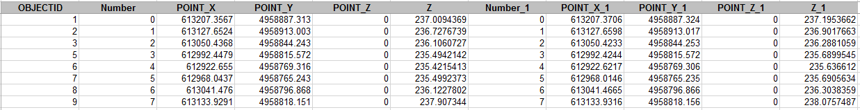 |
| Table 1: The output from the Table to Excel tool. |
 |
| Table 2: The distance between the GCP locations on the images generated with and without the use of GCPs |
 |
| Table 3: The total 3-Dimensional distance between the locations in table 1. |
 |
| Table 4: The horizontal RMSE, vertical RMSE, and average value for table 3. |
The error between the two surfaces was rather minor, yet noticeable in certain parts of the images. The horizontal RMSE was 1.406 cm, slightly less than its pixel size of 1.666cm (Table 4). The vertical RMSE was substantially higher, at 18.78cm.
 |
| Image 1: The locations of the GCPs throughout Litchfield Mine. |
The images appeared identical at first, but closer inspection revealed discrepancies between the two (Image 2).
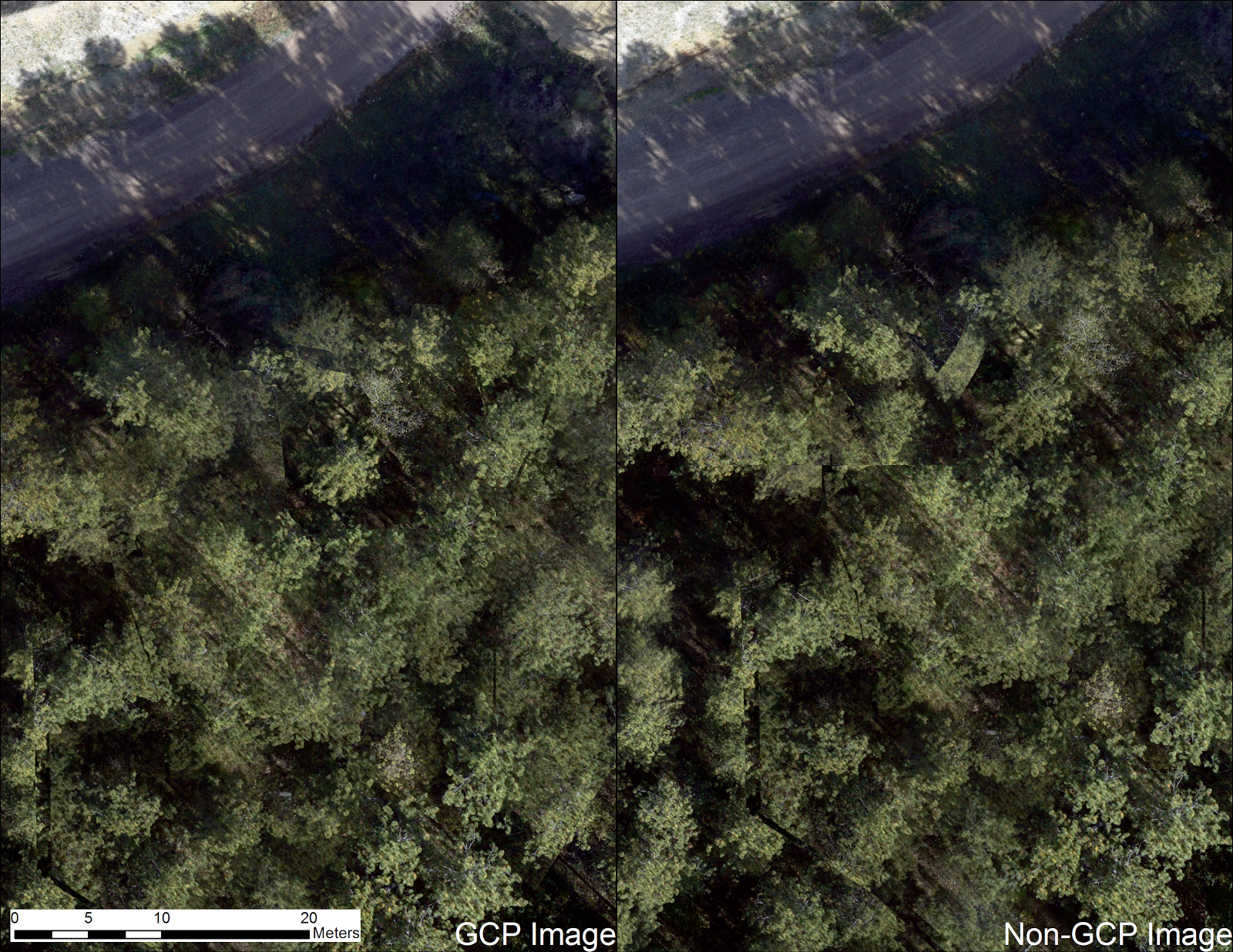 |
| Image 2: Notice the discrepancy between the two images 1/3rd from the top of the image. |
 |
| Image 3: Elevation error and GCP locations. |
At first I believed this increase in error was caused by the distance, but upon further inspection it seems the error is related to the type of feature (Image 4).
 |
| Image 4: Elevation error and feature type. |
Conclusion:
The RMSE calculations indicated Pix4D's mosaics generated without GCPs have horizontal error less than the pixel size. This will be very useful for helping determine when GCPs are necessary in the future. The high vertical RMSE from the Non-GCP imagery, indicates that GCPs are truly important when recording elevation.
Sunday, February 21, 2016
Processing Imagery with Pix4D
Introduction:
Pix4D is a software package that allows for automated
bundle-block adjustment to be performed on UAS imagery. The software is
extremely powerful, and can generate point clouds and orthomosaics from images,
without the aid of a human technician.
The program is powerful, but needs data to be collected
within certain parameters. When capturing any imagery, Pix4D needs at least 75%
frontal overlap, and at least 60% side overlap for it to derive useful results.
The necessary overlap percentages change depending on the surface. When
capturing surfaces covered in sand or snow, Pix4D needs at least 85% frontal
overlap and at least 70% side overlap.
When flying over fields, it requires the same overlap percentages as
snow or sand, and also requires the flights to be done at lower altitudes, as
it will increase the visual content.
Pix4D’s rapid check feature can be used to assess the quality of
collected imagery in the field. When a study area requires multiple flights, it
is important to ensure there is enough overlap between flight plans and that
the images are captured with similar sun direction. For Pix4D to process
oblique images, it is necessary for images to be captured first at a 45-degree
angle and for additional images to be captured with increased flight heights
and decreased angles. Ground Control Points (GCPs) are points within the area
of interest with known coordinates. They increase the accuracy of Pix4D’s
results by placing the model on its exact position on Earth’s surface. Once data
are brought into Pix4D, the “Initial Processing” step can be performed. Initial
processing generates a quality report, defining the accuracy criteria and
average ground sampling distance of the project.
Methods:
I used Pix4D to process imagery captured with two different
sensors, a Canon SX260 and the Sentek GEMs. The SX260 has built-in GPS, meaning
it records the cameras spatial location in the metadata of each image as they
are captured. The GEMs records the locational information in a slightly different
manner, requiring the images to be processed using Sentek’s software in order
to obtain the images locational information. In order to process the images, I
first needed to create a new project, and specify the project’s file location. Next, I added images to the project from
their folder locations. When processing GEMs imagery, it is important not to
accidentally include photos from both the visible spectrum and NIR spectrum,
but rather process them individually. After the images have been selected, the
next step is to make sure their geolocation information is correct and that the
correct camera model is selected. As I said earlier, the SX260’s geolocation
information is saved within each image, so the screen should show a green check
mark next to the geolocation and orientation status. The GEMs requires its
geolocation information to be imported from a spreadsheet before it can be
processed. The GEMs sensor also requires its characteristics (focal length,
sensor size) to be entered in manually before any processing can occur. After
all of the parameters have been entered, the project is created.
After the projects were created, I performed initial
processing to determine the quality of the collected imagery. The SX260 imagery
consisted of 108 total images, of which 105 were used. The three removed images
appear to have been captured as the UAS was ascending, leading to pixel
distortion and less accurate geolocation (Figure 1).
 |
| Figure 1: Images removed when processing the Canon SX260 flight |
The areas between flight lines had
slightly less overlap than where the UAS turned between flight lines (Figure 2).
 |
| Figure 2: Number of overlapping images taken with the SX260 |
The GEMs
imagery consisted of 146 total images, of which 142 were used. The four removed
images appear to have been captured over a line of trees with intense
shadows…likely causing the software to have difficulty identifying matching pixels (Figure 3).
 |
| Figure 3: Images removed when processing the GEMs flight. |
The area covered by the removed images is where the flight plan has lowest
overlap (Figure 4).
 |
| Figure 4: Number of overlapping images taken with the GEMs |
After analyzing the quality report, I continued processing
the data through the “Point Cloud Densification” and “DSM and Orthomosaic
Generation” steps. Once the point clouds were generated it was possible to
perform 2D and 3D calcuations from the point cloud as well as create a 3D fly-by animation (Figures 5,6).
 |
| Figure 5: Calculating the total area of the community garden from the GEMs point cloud. |
 |
| Figure 6: Calculating the volume of a shed at the community garden from the GEMs point cloud |
Results:
The orthomosaics and DSMs were generated for the
SX260 and GEMs at 1.44cm GSD and 2.62cm GSD, respectively. I measured a known
distance (the 100 yard section of the running track) on the SX260 point cloud,
in order to perform a basic assessment of spatial error. When measured, Pix4D
measured the track’s length to be 100.68 meters or 110.104987 yards, 10%
greater than its actual length (Figure 7).
 |
| Figure 7: When measured in Pix4D, the track is 100.68m long. |
It is currently impossible for me to currently
ascertain the spatial accuracy for other parts the imagery, as I don’t have any
GCPs or other known distances. The DSM generated from the GEMs had elevation
values 30 meters lower than the ground surface. This error is due to the
internal GPS’s method of recording elevation not matching the parameter I set
when entering the images into Pix4D.
 |
| Figure 8: The Orthomosiac and DSM generated from the SX260 |
 |
| Figure 9: The orthomosaic and DSM generated from the GEMs |
 |
| Figure 10: a. This image was resampled using the Natural Neighbors method (left). b. This image was resampled using Bilinear Interpolation (right). |
 |
| Figure 11: a. This image was resampled using the Natural Neighbors method (left). b. This image was resampled using Bilinear Interpolation (right). |
Pix4D automates the photogrammetric process, allowing for relatively fast processing of UAS imagery, and does so rather well. The derivatives generated without GCPs appeared to be true to reality, and didn't feature any major distortion. The program has incredible capabilities, however, attention should still be paid to accuracy.
Saturday, February 13, 2016
Use of the GEMs Processing Software
Introduction:
The Sentek Geo-localization and Mosaicing Sensor (GEMS) is a VIS/NIR combination sensor that was designed for the generation of vegetation health indexes. It uses two cameras mounted side-by-side in order to capture the images simultaneously.
What does GEMs stand for? Geo-localization and Mosaicing System.
Look at figure 3 in the hardware manual and name what the GSD and pixel resolution are for the sensor. Why is that important for engaging in geospatial analysis. How does this compare to other sensors? The GEMS' GSD is 2.5cm @ 200 ft and the camera resolution is 1.3mp ~ (1280x1024). A Canon SX260 has a GSD of 2.06cm @ 200ft and the camera resolution is 12.1mp ~ (4256x2848).
How does the GEMs store its data. The data are stored on a USB storage device.
What should the user be concerned with when mounting the GEMs on the UAS? The sensor should be: maximally flat, away from magnets, in a vibration free location, and shielded from electromagnetic interference.
Examine Figures 17-19 in the hardware manual and relate that to mission planning. Why is this of concern in planning out missions? The sensor has an extremely narrow field of view, which requires many closely spaced flight lines are required to cover even an extremely small area.
Write down the parameters for flight planning software (page 25 of hardware manual). Compare those with other sensors such as the Cannon SX260, Cannon S110, Nex 7, DJI phantom sensor, and Go Pro.
Software Manual:
Read the 1.1 Overview section. Then do a bit of online research and answer what the difference between orthomosaic and mosaic for imagery (orthorectified imagery vs. georeferenced imagery). Is Sentek making a false claim? Why or why not? Sentek is making a false claim, as their imagery is not actually an orthomosaic. An orthomosaic is a collection of images that were all rectified into the same plane using their z values, so the distance between two points on the image is exactly the same as their ground distance. This allows for measurements to be recorded from the images. A georeferenced mosaic is a collection of images that were combined by matching pixel values with one another, and using their relative coordinates to assign their locations in the resulting image.
What forms of data are generated by the software? RGB, NIR, and NDVI imagery.
How is data structured and labeled following a GEMs flight? What is the label structure, and what do the different numbers represent? The data are structured by the time of the flight, with the first value being the "GPS week" the flight was conducted. The subsequent values represent the hours, minutes, and seconds of the GPS week at the moment the flight started.
What is the file extension of the file the user is looking to run in the folder? The user is looking for the '.bin' extension.
The Sentek Geo-localization and Mosaicing Sensor (GEMS) is a VIS/NIR combination sensor that was designed for the generation of vegetation health indexes. It uses two cameras mounted side-by-side in order to capture the images simultaneously.
What does GEMs stand for? Geo-localization and Mosaicing System.
How does the GEMs store its data. The data are stored on a USB storage device.
What should the user be concerned with when mounting the GEMs on the UAS? The sensor should be: maximally flat, away from magnets, in a vibration free location, and shielded from electromagnetic interference.
Examine Figures 17-19 in the hardware manual and relate that to mission planning. Why is this of concern in planning out missions? The sensor has an extremely narrow field of view, which requires many closely spaced flight lines are required to cover even an extremely small area.
Write down the parameters for flight planning software (page 25 of hardware manual). Compare those with other sensors such as the Cannon SX260, Cannon S110, Nex 7, DJI phantom sensor, and Go Pro.
Camera
|
Sensor Resolution
|
Sensor Dimensions
|
Horizontal FOV (degrees)
|
Vertical FOV (degrees)
|
Focal Length
|
GEMS
|
1280 x 960 pixels
|
4.8x3.6mm
|
34.622
|
26.314
|
7.70mm
|
Canon SX260
|
4000 x 3000
|
6.30 x 4.72mm
|
69
|
54.5
|
4.5mm
|
Canon S110
|
4000 x 3000
|
7.60 x 5.70mm
|
73
|
58
|
5.2mm
|
Sony Nex7
|
6000 x 4000
|
23.6 x 15.7mm
|
67.4
|
47.9
|
18mm
|
DJI Phantom
|
4000 x 3000
|
6.30 x 4.72mm
|
81.7
|
66
|
3.6mm
|
GoPro
|
4000 x 3000
|
6.30 x 4.72mm
|
122.6
|
94.4
|
2.98mm
|
Software Manual:
Read the 1.1 Overview section. Then do a bit of online research and answer what the difference between orthomosaic and mosaic for imagery (orthorectified imagery vs. georeferenced imagery). Is Sentek making a false claim? Why or why not? Sentek is making a false claim, as their imagery is not actually an orthomosaic. An orthomosaic is a collection of images that were all rectified into the same plane using their z values, so the distance between two points on the image is exactly the same as their ground distance. This allows for measurements to be recorded from the images. A georeferenced mosaic is a collection of images that were combined by matching pixel values with one another, and using their relative coordinates to assign their locations in the resulting image.
What forms of data are generated by the software? RGB, NIR, and NDVI imagery.
How is data structured and labeled following a GEMs flight? What is the label structure, and what do the different numbers represent? The data are structured by the time of the flight, with the first value being the "GPS week" the flight was conducted. The subsequent values represent the hours, minutes, and seconds of the GPS week at the moment the flight started.
What is the file extension of the file the user is looking to run in the folder? The user is looking for the '.bin' extension.
What is the basis of this naming scheme? Why do you suppose it is done this way? Is this a good method. Provide a critique. This naming scheme is based on the time the flight began. This is done so no folders have the same names. The only negative of this naming convention, is that it is difficult to interpret the meaning of the folders unless the names are converted to local time.
Explain how the vegetation relates to the FC1 colors and to the FC2 colors. Which makes more sense to you? Now look at the Mono and compare that to the vegetation. The areas with high NDVI values have higher reflectance values in the NIR spectrum than in the visible spectrum. Areas with lush vegetation have higher NIR reflectance and are shown as having higher NDVI values than areas of drier vegetation. Areas with high NDVI values in FC1 are shown in red, and low values are shown in blue. Areas with high NDVI values in FC2 are shown in green, and low values are shown in red. The color ramp used by FC2 makes more logical sense than the color ramp used by FC1, as people are more likely to associate green with healthy vegetation, and red with unhealthy vegetation.
Now go to section 4.5.5 and list what the two types of mosaics are. Do these produce orthorectified images? Why or why not? The two mosaic types are 'Fast' and 'Fine'. Neither method produces orthorectified images, because they don't take the images elevations into account.
Generate Mosaics. Be sure to check all the boxes so you compute NDVI, use the default color map, perform fine alignment. Make sure you uncheck use GPU acceleration. Describe the quality of the mosaic. Where are there problems. Compare the speed with the quality and think of how this could be used. The mosaic generation is a relatively quick process, but its results are less than stellar. There are some errors where linear features show discontinuity, but the quality is good for the fast processing time.
Navigate to the Export to Pix4D section. What does it mean to export to Pix4D? Run this operation and look at the file. What are the numbers in the file used for? (Hint: you will use this later when we use Pix4D) The Export to Pix4D operation creates a '.csv' file which holds the coordinate information for all of the images, which will be used when processing the imagery in Pix4D.
Go to section 9.6 on Geo-tif. What is a geotif, and how can it be used? A geotiff is a geo-referenced mosaic, and can be easily added to any GIS tool for additional processing or display.
Go into the Tiles folder and examine the imagery. How are the geotifs different than the jpegs? The geotiffs have their coordinate data saved within their files, which allows for their easy display in GIS software.
Use what you learned from last week to describe patterns on each map.
Part 4: Conclusions
Go into the Tiles folder and examine the imagery. How are the geotifs different than the jpegs? The geotiffs have their coordinate data saved within their files, which allows for their easy display in GIS software.
 |
| Figure 1: RGB Imagery |
The RGB images show distinctive differences in lighting in the mosaiced images, specifically where flight lines overlap. This is seen as vertical striping down across the images (Figure 1).
 |
| Figure 2: NIR Imagery |
The NIR images show substantially less contrast and detail in highly shadowed areas. These areas are the same striped areas visible in the RGB imagery (Figure 2).
 |
| Figure 3: Mono NDVI Imagery |
The Mono NDVI images have values that seem to have been skewed by the shadowed regions of the NIR imagery, as those regions have relatively lower reflectance values than other regions of the images (Figure 3).
 |
| Figure 4: NDVI FC1 Imagery |
The NDVI FC1 images further exaggerate the negative emphasis the shadowed regions of the images had on the overall output NDVI values. The shadows completely eliminated the scale from the NDVI calculations,
 |
| Figure 5: NDVI FC2 Imagery |
The NDVI FC2 images show healthy vegetation in green and unhealthy vegetation and other objects in red. The shadowing of the NIR images, again ruined the scale of the pond imagery, showing similar vegetation as having completely different values.
Part 4: Conclusions
The GEMs software and sensor seem like wonderful equipment, however, in practice the results are underwhelming. The software can produce a mosaiced image incredibly quckly, something of high value in the field, however, it sacrifices quality for speed.
The sensor itself has a narrow field of view, a quality that reduces the distortion in its captured images. The narrow field of view is a double-edged sword, and requires more flight lines to cover the same area as a camera with a wider field of view.
The GEMs system seems like a wonderful idea, but becomes limited by certain hiccups. Although it shoots VIS and NIR imagery simultaneously, the images are kept seperate, rather than combined into a multiband image. This limits their usability, and limits the capabilities of Pix4D's photogrammetry algorithms. The sensor's small field of view and tiny sensor both combine to make it an incredibly cumbersome sensor to fly, as it requires incredibly longer flight times when compared to other sensors. The fact that its weight is comparable to the other - higher resolution sensors, and that it costs substantially more than the other sensors both speak against its use.
The GEMs system seems like a wonderful idea, but becomes limited by certain hiccups. Although it shoots VIS and NIR imagery simultaneously, the images are kept seperate, rather than combined into a multiband image. This limits their usability, and limits the capabilities of Pix4D's photogrammetry algorithms. The sensor's small field of view and tiny sensor both combine to make it an incredibly cumbersome sensor to fly, as it requires incredibly longer flight times when compared to other sensors. The fact that its weight is comparable to the other - higher resolution sensors, and that it costs substantially more than the other sensors both speak against its use.
Subscribe to:
Posts (Atom)